Basic tutorial
This basic tutorial covers the basic functions of the MAxPy framework. By the end of it, you will be able to understand how MAxPy works and its available tools. Then, you can use the framework to develop and optimize your own circuits.
To follow this tutorial, you can create and edit the files as requested, or you can use the code available here.
Note
Basic means base, not easy! =D
The problem
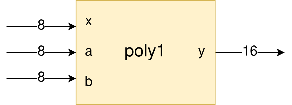
Suppose you want to make a hardware accelerator for a Polynomial Function of Degree 1: a linear function. The operation is pretty straightforward: the \(y(x)\) output for any given \(x\) input is the factor \(a\) times the \(x\) input plus factor \(b\), as shown in the equation below.
As the equation shows, we can see that the linear function is performed by two arithmetic operations: one sum and one multiplication.
Now we are going to make some assumptions for our application:
From now on, we will call our linear function circuit as poly1.
The circuit is going to have 3 inputs (x, a and b), and only one output (y);
Each of the three inputs will be 8 bits wide, being the MSB the signal bit (values ranging from -128 to 127);
To cover all possibilites for data inputs, the output will be 16 bit wide;
The application in which the linear function hardware accelerator will be used tolerates an error range of 10%. To measure the error, we are going to use the Mean Absolute Percentage Error - the MAPE.
Taking these assumptions into account, we can draw the following block diagram which represents our hardware accelerator:
RTL design
Let’s write the Verilog description of our linear function hardware accelerator. Create anywhere in your system a directory called poly1, in which will put all design files used in this tutorial. From now on, we will call this the working directory. Inside the working directory, create a subdirectory named rtl, and create a new text file called poly1.v.
poly1
└── rtl
    └── poly1.v
The following code is the hardware description of our circuit, written in Verilog:
module poly1(a, b, x, y);
    input signed [7:0] a, b, x;
    output signed [15:0] y;
    assign y = a*x + b;
endmodule
Converting from Verilog to Python
Now we are going to compile the poly1 module in MAxPy, but without any optimizations or approximations for now. The goal at this point is to make a functional module that we can use to write our testbench.
Create a run1.py file inside the working directory:
poly1
├── rtl
│   └── poly1.v
└── run1.py
The run1.py is a Python script, which will be used to invoke MAxPy’s command. The content of the run1.py is the following:
from MAxPy import maxpy
circuit = maxpy.AxCircuit(top_name="poly1")
circuit.rtl2py(target="exact")
Notice that this script performs only three commands:
It imports the MAxPy framework into Python
It creates an instance of
AxCircuitclass and stores it in thecircuitobject, passing the RTL design’s top circuit name to thetop_nameparameter (this is important: the top circuit name passed here has to be the same declared in the Verilog module)It runs the
rtl2pymethod to convert the RTL design into a Python module, passing the valueexactto thetargetparameter
Now it’s time to get MAxPy running! Run the following lines in the terminal:
python run1.py
If everything is fine, you should see a terminal output like the following. In case of any error, please check the Installation section and review every step of this tutorial.
MAxPy - Version 0.0.1

------------------------------------------------------------------------------------
>>> MAxPy rtl2py: converting Verilog RTL design "poly1" into Python module
> Base "rtl", Target "exact"
> Start: 04-03-2023 22:48:39
> Synth
> Netlist estimated area: 110.887
> Netlist estimated power = 5.066 uW
> Netlist estimated maximum delay = 127.195 nS
> Verilator
> C++/Python Wrapper
> C++ compilation
ninja: Entering directory `poly1_exact/'
[11/11] Linking CXX shared module poly1.cpython-310-x86_64-linux-gnu.so
>> 3.8 seconds
> Module check (should print module's name)
> poly1
> End: 04-03-2023 22:48:43
>>> Circuit "poly1" converted successfully!
Let’s take a look on our working directory to see what changes after a successful compilation:
poly1
├── rtl
│   └── poly1.v
├── poly1_exact
│   ├── source
│   ├── netlist_yosys
│   ├── CMakeFiles
│   ├── CMakeLists.txt
│   ├── build.ninja
│   ├── *.log
│   └── poly1.cpython-310-x86_64-linux-gnu.so
└── run1.py
A directory named poly1_exact is created. Notice that this name is made combining the top name of the RTL design with the target parameter passed in the rtl2py command. Inside it there are several other files and directories:
poly1.cpython-310-x86_64-linux-gnu.so: this is the final product of any successful conversion of a Verilog design to Python. This .so file is a shared library that had been compiled based on our circuit funcionality, and then can be loaded into any Python script. Shortly we’ll check how to do so.netlist_yosys/: it stores the gate-level netlist generated by the logic synthesis tool. Even if thertl2pycompilation is being performed in the RTL level, a gate-level netlist is generated for resources estimation purposes (area, power and timing). If no specific synthesis tool is provided, the default one is Yosys.source/: directory which contains the C++ source files generated from the Verilog to C++ conversion process (using Verilator), plus the C++ to Python wrapper (generated by MAxPy using Pybind11). This directory exists only for the C++ compilation process, or eventally for debugging purposes. Normally the user doesn’t need to care about it.CMakeFiles/,CMakeLists.txtandbuild.ninja: the compilation of the final Python module is performed combining CMake and ninja build system. The user shouldn’t need to care about them.Log files: every step of the
rtl2pyprocess creates a*.logfile with useful debug information.
Writing a testbench
Now that we have a shared library, we are going to import it into another Python script to perform the simulation and get the evaluation of our circuit: this is the testbench. Create a tesbench.py in the working directory:
poly1
├── rtl
│   └── poly1.v
├── poly1_exact
│   ├── (...)
│   └── poly1.cpython-310-x86_64-linux-gnu.so
├── run1.py
└── testbench.py
Equally important as the shared libraries obtained from the rtl2py process, the testbenchs are very important in MAxPy. With them you are able to simulate your circuit operation in a Python environment without the need of a dedicated Verilog simulator. The benefits of doing so are:
Importing and exporting data to and from the circuit is way more friendly in a Python environment than it is in dedicated Verilog simulators.
Use of advanced Python libraries to get quality metrics within the simulation loop.
Feed simulation data, such as switching activity, back to MAxPy to get further optimizations with Approximate Computing Techniques.
Change the circuit behaviour during simulation using the cycle-accurate switching activity data available in every circuit on MAxPy.
However, the testbench needs to be carefully designed to meet both MAxPy’s required stucture and also the own circuit funcionality.
Take a look at the code from testbench.py showed below:
import importlib
from MAxPy import results
from sklearn.metrics import mean_absolute_percentage_error
from sklearn.metrics import mean_absolute_error
from sklearn.metrics import accuracy_score

def testbench_run(ckt=None, results_filename=None):
    lin = ckt.poly1()
    rst = results.ResultsTable(results_filename, ["mape", "mae", "accuracy"])
    print(f">>> testbench init - circuit: {lin.name()}, area: {lin.area}, parameters: {lin.parameters}")
    y_true = []
    y_pred = []
    for a in range(-128, 128):
        lin.set_a(a)
        for b in range(-128, 128):
            lin.set_b(b)
            for x in range(-128, 128):
                lin.set_x(x)
                lin.eval()
                y_out = lin.get_y()
                if y_out & 0x8000:
                    y_out ^= 0xffff
                    y_out += 1
                    y_out *= -1
                y_ref = int(a*x) + b
                if y_ref != 0:
                    y_true.append(y_ref)
                    y_pred.append(y_out)
                count += 1

    mape = mean_absolute_percentage_error(y_true, y_pred)
    mae = mean_absolute_error(y_true, y_pred)
    accuracy = accuracy_score(y_true, y_pred)
    rst.add(lin, {"mape": mape, "mae": mae, "accuracy": accuracy})
    print(f"> mape: {mape:.4f}, mae: {mae:.4f}, accuracy: {accuracy:.4f}")
    print(">>> testbench end")
    if mape < 0.1:
        prun_flag = True
    else:
        prun_flag = False
    return prun_flag, lin.node_info


if __name__ == "__main__":
    mod = importlib.import_module(name="poly1_exact.poly1")
    testbench_run(ckt=mod, results_filename="testbench_dev.csv")
Every testbench script should look like this one! Basically, a MAxPy testbench script has two sections: the __main__ part at the bottom, and the testbench_run function.
The reason for putting the testbench routine in a separate function is that the function can be called when MAxPy is running its automated process (we’ll get into that shortly).
Also, the main part below is needed when we are designing the testbench itself, so once we have compiled a shared library, we can just run the testbench.py script without the needed of running the compilation again.
__main__: no big deal in this. It just loads a compiled shared library and calls thetestbench_runfunction, passing the shared library as argument. Notice that in this tutorial we are using thepoly1_exact.poly1compilation, but it could be any other name created in the design process.testbench_run: is the testbench routine. Here some things need to happen:The shared library is passed to the
testbench_runfunction via theckt(circuit) parameter. Then we need to make an object of the shred library so we can manipulate it. In this example, the object is calledlin(for linear), but the can be any other.def testbench_run(ckt=None, results_filename=None): lin = ckt.poly1()
We need to create an object of a MAxPy internal structure for results recording. This structure is called
ResultsTable, and it is instantiated at therstobject. Notice that we are passing a list of strings as arguments. Each string in this list represents a quality metric used in this circuit. As we stated at the begining of this tutorial, the chosen quality metric is the MAPE, so we are passing the["mape"]to theResultsTableobject. In spite of only one quality metric being allowed, we are adding two more quality metrics: the Mean Absolute Error (MAE) and the Accuracy Score. You can add as many parameters as you want.rst = results.ResultsTable(results_filename, ["mape", "mae", "accuracy"])
You can find information about these quality metrics in the following links:
This is a basic tutorial about how to use the MAxPy framework. The polynomial function application does not intend to be a real world application. Perhaps the chosen quality metrics are not the best fit for evaluating a polynomial function. If you have any suggestion that would fit better as example, please let us know - check the Contact page.
To apply values to the inputs of the circuit, we must use the
setfunctions. For every circuit input, MAxPy create a method in the shared library called set_ plus the name of the input. For example, as we have instantiated our circuit at thelinobject, we can write to the \(a\), \(x\) and \(b\) inputs by using the following methods:lin.set_a(value),lin.set_b(value)andlin.set_x(value). The values applied to the inputs must respect the bit width. For example, for an 8 bit input, the value must be in the range from 0 to 255. Any value outside of this range will throw an error and the execution will stop.After setting all input values, it is needed to call the
lin.eval()method. This is a default method from the Verilator tool. It’s purpose is to update all the circuit with the new input values, so we can get the output values.To get values from outputs, we need to use the
getmethods created by MAxPy for each output. In this application, we have only the \(y\) output, and we can access its value using thelin.get_y()function. Careful attention must be payed when dealing with negative numbers. The representation used in the circuit is regarding the bit width declared in the RTL description. For example, in a signed 8 bit output, a value of 0x80 represents the -128 value. If you use thelin.get_y()and load the result in anintvariable in Python, it will be simply considered as +128 (this happens because in 8 bit, the signal is represented in the bit number 7; in a Python application, the default int bit width is 32, so the signal is represented in the bit number 31). In this example, we used the following code to convert an 8 bit negative number to a 32 bit negative number:y_out = lin.get_y() if y_out & 0x8000: y_out ^= 0xffff y_out += 1 y_out *= -1
Also, regarding the tesbench loop, we have chosen to use all possibilities for the inputs: \(a\), \(x\) and \(b\), each one of them being 8 bit wide. This results in a set of 16,777,216 combinations, which may take some time to process (a few minutes) depending on the host system. Again, as this is not intended to be a real application, maybe to check every input possibilities could not be the best approach. Each application should consider which is the best way to evaluate the results.
The reference value is generated by the following function. Both the
y_refandy_outvalues are stored in separate arrays, so at the end of the loop we can use whichever method to calculate the quality metrics.y_ref = int(a*x) + b
The following section shows how a MAxPy testbench must end. The
testbench_runfunction must return two values: a boolean flag indicating whether the circuit should be further optimized, and the node information after the simulation was performed. This return values are needed when MAxPy is running in the automated loops, so it is able to know when to stop to perform optimizations if the quality metrics had reached a lower level than expected.if mape < 0.1: prun_flag = True else: prun_flag = False return prun_flag, lin.node_info
Exploring Approximate Arithmetic Blocks
Now that we have a working testbench able to run a complete simulation and to generate the desired quality metrics, suppose we want to explore a little our poly1 circuit.
One thing that MAxPy allows to do is to replace basic arithmetic blocks for approximate ones.
The MAxPy Project has a library of Approximate Arithmetic blocks, which is available at the AxArith repository.
Now let’s get back to the poly1 working directory. We are going to keep the rtl directory and the run1.py script as they are.
We’ll create then a new directory: the rtl_param. Inside this directory we’ll create a new RTL description, but with some differences that we’ll see shortly. Also, we’ll create the run2.py script, which is going to contain the MAxPy’s instruction for exploring arithmetic blocks.
poly1
├── rtl
│   └── poly1.v
├── rtl_param
│   └── poly1.v
├── poly1_exact
│   └── ...
├── run1.py
└── run2.py
MAxPy has a feature for text replacement in Verilog source files. Whenever we want to evaluate any circuit with variations at some specific part, we can write the RTL source using the [[param]] notation. The main thing here is the double brackets ([[ and ]). The word param inside the brackets acts as a variable name. This sort of variable will be replaced for value defined in the run2.py script.
Back to the poly1 application: it has two arithmetic operations: a multiplication and a sum.
module poly1(a, b, x, y);
    input signed [7:0] a, b, x;
    output signed [15:0] y;
    wire signed [15:0] p;
    [[MULTIPLIER_TYPE]] #(16, [[MULTIPLIER_K]]) mult1 (a, x, p);
    [[ADDER_TYPE]] #(16, [[ADDER_K]]) sum1 (p, b, y);
endmodule
In the above RTL description, instead of just assigning that y = a*x + b;, we are spliting this line into two other: the first calls a submodule with name [[MULTIPLIER_TYPE]], passing as parameters 16 as bit width and [[MULTIPLIER_K]] as approximation factor. The inputs of the multiplier submodule are connected to the a and x inputs, and the output is connected to the wire named p. The following lines calls another submodule called [[ADDER_TYPE]], passing as parameters 16 as bit width and [[ADDER_K]] as approximation factor. The inputs of the adder submodule are connected to the p wire and the b input, while the output of this sum is connect directly to the y output.
Below we can see the run2.py code:
from MAxPy import maxpy
from testbench import testbench_run

circuit = maxpy.AxCircuit(top_name="poly1")
circuit.set_testbench_script(testbench_run)

circuit.set_group("study_no_1")
circuit.set_synth_tool(None)
circuit.set_results_filename("output.csv")
circuit.parameters = {
    "[[MULTIPLIER_TYPE]]": ["LoBa", "Roba", "Drum", "Tosam"],
    "[[MULTIPLIER_K]]": ["1", "2", "3"],
    "[[ADDER_TYPE]]": ["copyA", "eta1", "loa", "trunc0"],
    "[[ADDER_K]]": ["1", "2", "3", "4"],
}
circuit.rtl2py_param_loop(base="rtl_param")
Please notice the following:
Comparing to the
run1.pyscript, we do not have changes until the linecircuit.set_testbench_script(testbench_run); here we also need to import MAxPy into Python, instantiate an MAxPy object and set the testbench script to it.As we are going to compile a set of circuits for every combination of parameters, MAxPy allow to create a group using the line
circuit.set_group("study_no_1"). This line just puts all the generated in a subdirectory calledstudy_no_1. This name is arbitrary; any other name can be used to make it more significant to the application.The line
circuit.set_synth_tool(None)defines that we are not using the gate-level simulation in this exploration. This is a recommendation because RTL-level compilation and simulation is faster than gate-level. We can use the gate-level later and apply it only to the most promising circuits.We can set the output file name with the line
circuit.set_results_filename("output.csv"). Any name can be used.The most important part here is the
circuit.parametersvariable. We need to initialize a Python dictionary with the keys containing the same names of the parameters we used in the RTL description above. For each key, the value must be a list of strings containing every value we want for each parameter to assume.The command
circuit.rtl2py_param_loop(base="rtl_param")puts MAxPy running, automaticaly generating as much circuits as possible combinations for the parameters.
For the defined parameters in this example, a total of 192 circuits are generated. As we have defined a group called study_no_1, every generated circuit is put on its own directory inside the study_no_1 directory. The working directory will look like the following:
poly1
├── rtl
│   └── poly1.v
├── rtl_param
│   └── poly1.v
├── poly1_exact
│   └── ...
├── study_no_1
│   ├── poly1_LoBa_1_copyA_1
│   ├── poly1_LoBa_1_copyA_2
│   ├── poly1_LoBa_1_copyA_3
│   ├── poly1_LoBa_1_copyA_4
│   ├── poly1_LoBa_1_eta1_1
│   ├── poly1_LoBa_1_eta1_2
│   ├── poly1_LoBa_1_eta1_3
│   ├── poly1_LoBa_1_eta1_4
│   └── ...
├── run1.py
└── run2.py
Probabilistic pruning
Conclusion
The script names
run1.py,run2.pyandrun3.pyare completely arbitrary. You can choose any name you want to match what the script does.