Case Study: Sobel Edge Detection
This tutorial presents a more advanced tutorial for an actual application. Here we are going to focus more on the application and less on the MAxPy instructions.
The circuit studied here is an Approximate Sobel Operator used for Edge Detection in images. You can check the code for this study case here.
Sobel Basics
The Sobel Operator is used digital processing of images as an approximation to the Gradient Filter, which is needed in edge detection applications. It is composed by two 3x3 convolution masks, each representing the pixel gradient in both \(x\) and \(y\) directions. The below equation show the convolution masks used in the Sobel Operator.
For any give point of an image, the gradient’s magnitude is defined as following:
To reduce circuitry complexity, the gradient value can be approximated by the sum of the \(x\) and \(y\) components absolute values. This sum is then compared to an input threshold value, defining whether or not the given pixel represents an edge.
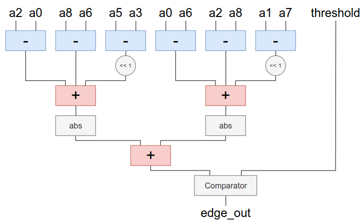
The image below depicts a block diagram for the Sobel Operator circuit. There we have 8 inputs for the pixels surrounding the pixel of interest (a0 to a8, skipping a4), one theshold input for the edge detection threshold, and an edge_out output, indicating if the pixel of interest is an edge or not.

Block diagram for the exact Sobel Operator
Quality Metrics
In this application, we are going to generate full images containing the edges of the original sample images. We need then compare the edge images generated by our Sobel Operator to the ones generated by a reliable reference, such as OpenCV. For image comparisson, we have choosen the Structural Simmilarity Index - the SSIM - as a quality metric. The SSIM can be defined as in the equation below, and there’s a Python implementation in the scikit-image toolbox.
Also, as we are getting boolean values for each pixel, we can check the accuracy of edge detection using the Accuracy Score defined in the equation bellow, where \(t_p\) is true positive count, \(t_n\) is true negative count, \(f_p\) if false positive count and \(f_n\) is false negative count.
RTL Exact Description
Now let’s get to the circuit description. The following code shows the Verilog description of the block diagram above with no further approximations other than the Sobel Operator already is compared to the Gradient Filter. It is placed in a file called sobel.v under the rtl directory inside the AxSobel working directory. This circuit can be compiled running the run_exact.py script.
module sobel_gradient(a1, a2, b1, b2, c1, c2, grad);
    input [7:0] a1, a2, b1, b2, c1, c2;
    output [10:0] grad;
    wire signed [8:0] g1, g2, g3;
    wire signed [9:0] g13, g22;
    wire signed [10:0] g;
    assign g1 = {1'b0, a1} - {1'b0, a2};
    assign g2 = {1'b0, b1} - {1'b0, b2};
    assign g3 = {1'b0, c1} - {1'b0, c2};
    assign g13 = g1 + g3;
    assign g22 = g2 * 9'd2;
    assign g = g13 + g22;
    assign grad = g[10] ? ~g+11'd1 : g;
endmodule

module sobel(p0, p1, p2, p3, p5, p6, p7, p8, threshold, edge_out);
    input [7:0] p0,p1,p2,p3,p5,p6,p7,p8;
    input [7:0] threshold;
    output edge_out;
    wire [10:0] gx, gy;
    wire [11:0] grad;
    sobel_gradient grad_x(p2, p0, p5, p3, p8, p6, gx);
    sobel_gradient grad_y(p0, p6, p1, p7, p2, p8, gy);
    assign grad = gx + gy;
    assign edge_out = grad > {4'd0, threshold} ? 1'b1 : 1'b0;
endmodule
You can find the full testbench script at this link. After running it with the exact circuit, we get the following output:
>>> testbench init
> circuit: sobel
> parameters: exact

> threshold: 127

> images list:
    > images/birds/birds.jpeg
    > images/butterfly/butterfly.jpg
    > images/fish/fish.jpg
    > images/mulholland/mulholland.jpeg

> processing image images/birds/birds
    > reference ok, loading (images/birds/birds_ref_bw.png)
    > result csv file ok, loading (sobel.csv)
    > dimension: W 1000 x H 563
    > loop init
    > loop end
> processing image images/butterfly/butterfly
    > reference ok, loading (images/butterfly/butterfly_ref_bw.png)
    > result csv file ok, loading (sobel.csv)
    > dimension: W 1024 x H 683
    > loop init
    > loop end
> processing image images/fish/fish
    > reference ok, loading (images/fish/fish_ref_bw.png)
    > result csv file ok, loading (sobel.csv)
    > dimension: W 1000 x H 667
    > loop init
    > loop end
> processing image images/mulholland/mulholland
    > reference ok, loading (images/mulholland/mulholland_ref_bw.png)
    > result csv file ok, loading (sobel.csv)
    > dimension: W 720 x H 720
    > loop init
    > loop end
> average result: ssim 0.9999, acc 99.99%
>>> testbench end
As we can see in the testbench output, four images are used as samples to evaluate the quality metrics of the exact verion of the Sobel Operator. For each one of the images, the testbench loop is performed and the quality metrics are accumulated. In the end, the average SSIM and Accuracy are calculated based on a comparisson with an edge image generated by OpenCV.
We’ve got a SSIM of 0.9999, and an Accuracy of 99.99%, proving that both our Verilog description and the testbench script are working good!
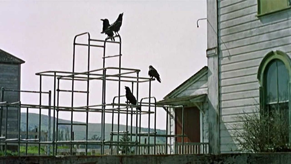
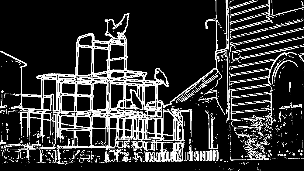
Here are some image samples of what is happening. We actually cannot see spot differences in edge detection with bare eyes.

Original image

OpenCV reference

Generated by the testbench script of out circuit in MAxPy
Note
You can try this with your own images! You just need to add them in the AxSobel/images directory, and then update the list in the testbench.py script.
Now that we have proved the Verilog description for the Sobel Operation is working with exact results, it’s time to tweak it a little to see how can we save some resources.
Using Approximate Adders
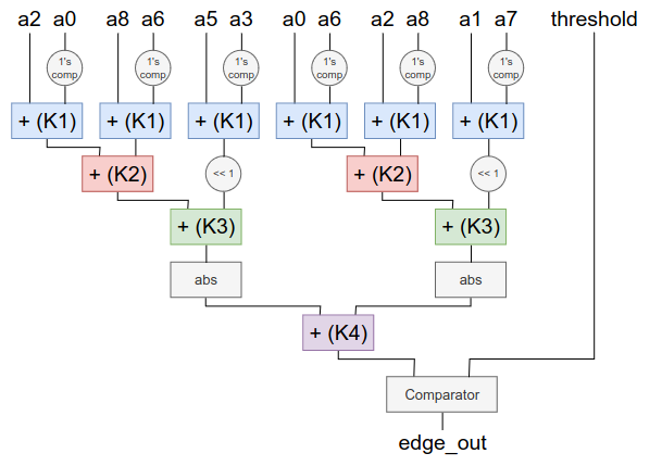
The following image shows the approach used to make an Approximate Sobel Operator using Approximate Adders in the sum operations. The sum operations had been divided into four groups regarding bit width. Each group has its own K factor.

Block diagram for the Sobel Operator with approximate adders
Note
K factor is the bit lenght that is going to be approximated in the operation. For example, if we are performing an addition of two 8 bit operands and a K factor of 4, the output’s higher bit part will be the exact sum of the 4 most sifnificant bits of each operand, while the lower bit part of the output will be approximate by the given method.
Note
The MAxPy Project has a library called AxArith, which is a collection of Approximate Arithmetic Blocks such as adders and multipliers.
The AxArith blocks are built in the MAxPy framework by default.
The following code is base on the RTL Exact Description shown above, but the sum operations had been replaced by submodules. But notice that the names of the submodules are not yet defined: they are being represented by some “variables” in the ``[[parameter]]`` format. The description below is placed in a file called sobel.v under the rtl_param directory inside the AxSobel working directory. This circuit can be compiled running the run_param.py script.
The run_param.py script defines the values for whose the [[parameters]] variables are going to be replaced. As the circuit has 11 sum operations, 4 different K factor levels, and six types of Approximate Adders, we are goint to have an amount of 14,406 circuits! MAxPy manages to build and simulate everyone of them, putting the results in a table so we can get the Pareto Front with the best results!
Note
Running the run_param.py script can take some time (hours long) depending on your system set-up!